Smooth, globally Polyak–Łojasiewicz functions are nonlinear least-squares

This is a companion post for an upcoming paper.

A function \(f \colon \Rn \to \reals\) with locally Lipschitz gradient is globally PŁ with parameter \(\mu > 0\) if \[ f(x) - f^* \leq \frac{1}{2\mu} \|\nabla f(x)\|^2 \] for all \(x\), where \(f^* = \inf_x f(x)\). Such functions are also called gradient dominated.

Polyak (1963) showed that the PŁ property is enough to ensure fast convergence of gradient descent to global minimizers. The optimization community has been interested in those functions ever since.

Example 1 Strongly convex functions are PŁ.

This is nice, but the whole point of PŁ is that it also spans nonconvex functions, and they can have nonisolated minimizers (whereas strongly convex functions have exactly one).

Example 2 Some nonlinear least-squares are PŁ.

Let \(f(x) = \frac{1}{2} \|A(x) - b\|^2\) for some \(A \colon \Rn \to \Rk\). The gradient is \(\nabla f(x) = \D A(x)^\top (A(x) - b)\), hence \[ \|\nabla f(x)\| \geq \sigmamin(\D A(x)) \, \|A(x) - b\| \geq \sigma \sqrt{2 f(x)} \] where \(\sigma := \inf_x \sigmamin(\D A(x))\). Notice \(f^* \geq 0\). If \(\sigma\) is positive, then \[ f(x) - f^* \leq \frac{1}{2\sigma^2} \|\nabla f(x)\|^2. \] (The condition \(\sigma > 0\) is sufficient but not necessary for \(f\) to be PŁ.)

The plan is to understand precisely what \(f\) and its set of minimizers can look like.

Punchlines

We start this post with limited regularity assumptions on \(f\).

Soon, we will require \(f\) to be smooth, that is, \(C^\infty\). For those, we have three main messages:

• All smooth globally PŁ functions \(f\) are nonlinear least-squares (!). See Theorem 1.

• The set of minimizers of \(f\) can be wild but not arbitrary, as characterized in Theorem 3.

• While \(f\) may not be convex, it is geodesically convex in disguise. See Theorem 4.

The set of minimizers \(S\)

The set of minimizers of a globally PŁ function \(f\) coincides with its set of critical points: \[ S = \{ x \in \Rn : f(x) = f^* \} = \{ x \in \Rn : \nabla f(x) = 0 \}. \] Clearly, \(S\) is closed in \(\Rn\). Let’s warm up with a few simple questions:

Question 1 Can \(S\) be a singleton?

Solution. Sure: just pick a strongly convex function.

Question 2 Can \(S\) be any affine space?

Solution. Sure: let \(f(x) = \frac{1}{2} \|Ax - b\|^2\) (linear least-squares) with \(\ker A \neq \{0\}\).

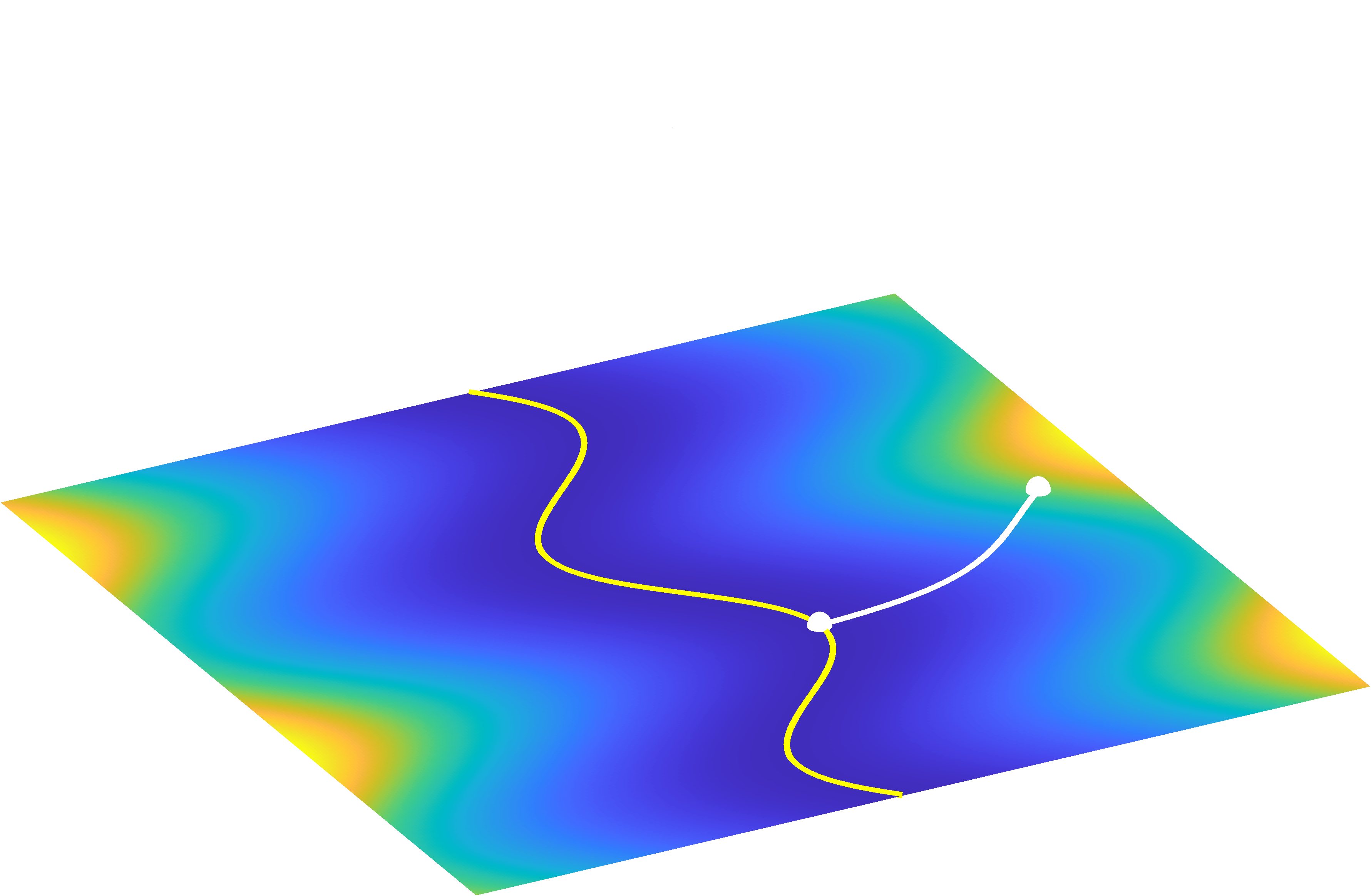
Question 3 Can \(S\) be squiggly (not flat)?

Solution. Yes: pick some \(g \colon \reals \to \reals\) (\(C^{1,1}_{\rm loc}\)) and let \(f(x) = \tfrac{1}{2}(g(x_1) - x_2)^2\). Then \(S\) is the graph of \(g\) in \(\reals^2\), and \(f\) is \(1\)-PŁ.

Example of a PŁ function on \(\reals^2\): \(f(x) = \tfrac{1}{2}(\sin(x_1) - x_2)^2\).

Question 4 Can \(S\) be empty?

Solution. No! This will become clear in the next section: running negative gradient flow from any point generates a trajectory that converges to some point, and that point must be a critical point.

We will find out more as we go.

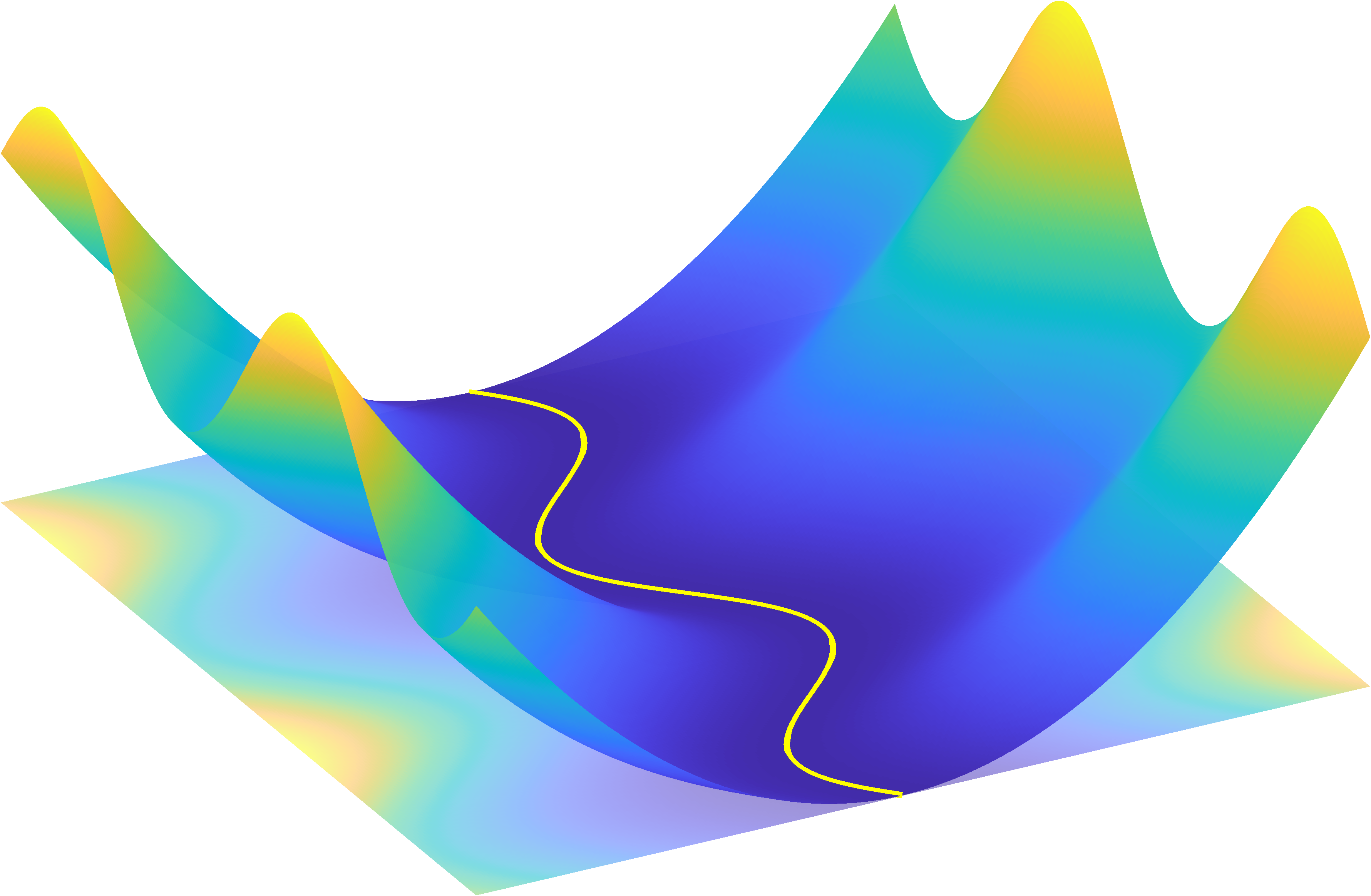
Flowing down \(f\) with \(\pi\)

Consider running negative gradient flow on \(f\), initialized at some point \(x_0 \in \Rn\): \[ x'(t) = -\nabla f(x(t)), \qquad x(0) = x_0. \] This ODE has a unique solution \(t \mapsto x(t)\), well defined for some interval of times around \(t = 0\).

This is why we assumed \(\nabla f\) is locally Lipschitz. If \(f\) is only \(C^1\), we might have \(f(x) = \tfrac{1}{2}(|x_1|^{3/2} - x_2)^2\) (indeed PŁ) for which negative GF initialized at \((0, 1)\) is not uniquely defined. To see this, check that \(f\) has the same value at both \((0, 0.573)\) and \((0.09, 0.6)\) and that positive GF initialized at either of them leads us to \((0, 1)\).

By a classical argument of Łojasiewicz and Otto and Villani (2000), the trajectory has finite length for \(t \geq 0\) (see below). This has two consequences:

1. The trajectory remains bounded, hence \(x(t)\) is defined for all \(t \geq 0\) (by the Escape Lemma).

2. The trajectory has a limit point for \(t \to \infty\).

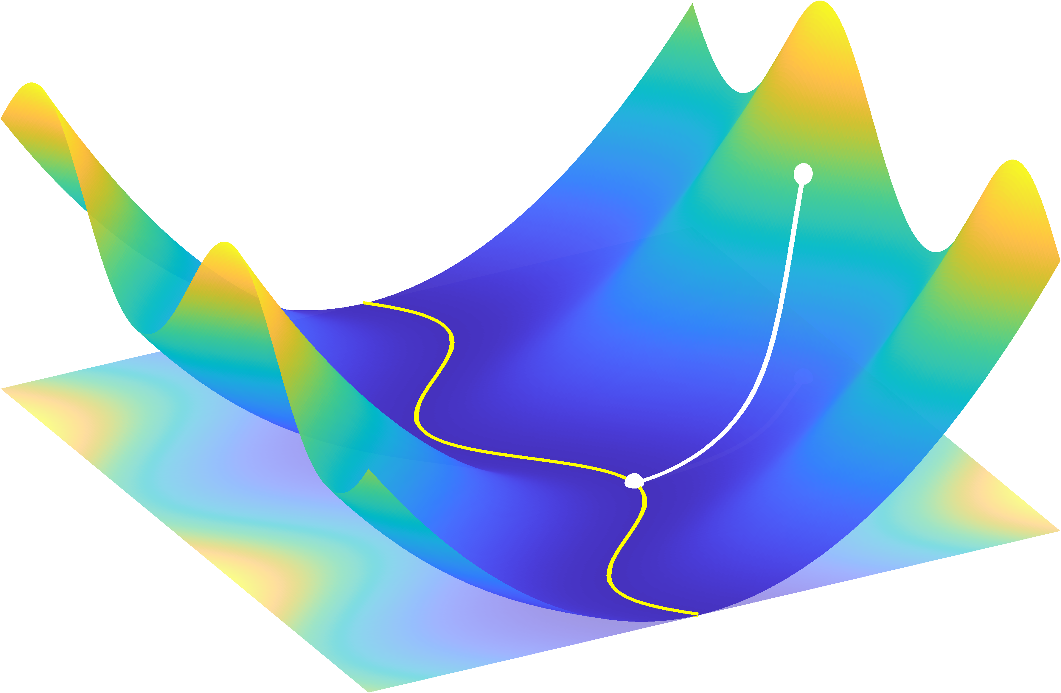
Let \[ \pi(x_0) := \lim_{t \to \infty} x(t) \] denote this limit. Clearly, it must be a critical point. Thus, \[ \pi \colon \Rn \to S \] is a well defined projection onto \(S\): we call it the end-point map.

 

Lemma 1 The GF trajectory has bounded length for \(t\) from 0 to \(\infty\): \[ \|x(t) - x(0)\| \leq \int_0^t \|x'(\tau)\| \, \dtau \leq \sqrt{\frac{2(f(x(0)) - f^*)}{\mu}}. \]

Proof. The classical argument defines \(h(t) = \sqrt{\frac{2(f(x(t)) - f^*)}{\mu}}\) and bounds the length of the trajectory as: \[\begin{align*} \int_0^t \|x'(\tau)\| \, \dtau & = \int_0^t \|\nabla f(x(\tau))\| \, \dtau \\ & = \int_0^t \frac{\|\nabla f(x(\tau))\|^2}{\|\nabla f(x(\tau))\|^{\phantom{2}}} \, \dtau \\ & \leq \int_0^t \frac{\|\nabla f(x(\tau))\|^2}{\sqrt{2\mu(f(x(\tau)) - f^*)}} \, \dtau \\ & = \int_0^t -h'(\tau) \, \dtau = h(0) - h(t) \leq h(0). \end{align*}\]

Topological implications

A first important observation is that:

Recall that for now we only assume the PŁ function \(f\) has a locally Lipschitz gradient.

Lemma 2 The end-point map \(\pi \colon \Rn \to S\) is continuous.

Proof (sketch). Negative gradient flow corresponds to a flow map \(\Phi\) defined such that \(x(t) = \Phi^t(x_0)\). Standard results show that \(\Phi^t \colon \Rn \to \Rn\) is continuous for all \(t \geq 0\). Given \(y \in \Rn\), we can choose \(t\) large enough such that \(\Phi^t(y)\) is close to \(S\). Also, \(\pi = \pi \circ \Phi^t\). Thus, \(\pi\) is continuous if it is so near \(S\). And indeed, near \(S\) the trajectories do not travel far (due to Lemma 1).

Question 5 Can \(S\) be disconnected?

Solution. No: \(S = \pi(\Rn)\) is the continuous image of a connected set, so it is connected.

Question 6 Can \(S\) be a circle in \(\reals^2\)?

Solution. No: there is no way to continuously deform \(\reals^2\) to a circle.

Consider any curve \(c\) which loops once around the circle for \(t \in [0, 1]\), with \(c(0) = c(1)\). Then, for each \(s \in [0, 1]\), the curve \(\gamma_s(t) = \pi((1-s)c(t))\) lives on the circle. As \(s\) goes from 0 to 1, \(\gamma_s\) gradually goes from looping around (since \(\gamma_0 = c\)) to being just a point (since \(\gamma_1(t) \equiv \pi(0)\)). This is impossible because the circle is not simply connected.

Gradient flow provides even more topological information about \(S\). For example:

Lemma 3 \(S\) is contractible, that is, it can be (internally) shrunk to a point.

Proof. We can shrink \(\Rn\) to (say) the origin with \(H(x, t) = (1-t)x\) for \(t \in [0, 1]\). For \(S\), consider \(G(x, t) = \pi(H(x, t))\): it’s continuous from \(S \times [0, 1]\) to \(S\) and for all \(x \in S\) we have both \(G(x, 0) = x\) and \(G(x, 1) = \pi(0)\) (one point in \(S\)).

A stronger statement holds: \(\Rn\) and \(S\) are homotopy equivalent. This is because \(\Phi^t\) brings all of \(\Rn\) down to \(S\), continuously, while keeping \(S\) fixed, so that \(\Rn\) (strongly) deformation retracts to \(S\).

At a high level, this means \(\Rn\) and \(S\) share many (though not all) topological properties.

Question 7 Can \(S\) be compact?

Solution. Sure (even though \(\Rn\) is not): \(S\) can be a singleton after all. But there’s more.

For example, the squared distance to the interval \([-1, 1]\) on the real line is \[ f(x) = \max(0, |x|-1)^2. \] This is PŁ and \(S = [-1, 1]\) is compact (not a singleton). Notice \(f\) is \(C^{1,1}\) but not \(C^2\). (There is more to say here, see (Garrigos 2023).)

Next, we impose more smoothness on \(f\). This changes the picture in interesting ways.

Let’s assume \(f\) is \(C^\infty\)

From now on, let us assume that \(f\) is globally PŁ and smooth. In particular, \(f\) has a Hessian and one can argue that the rank of \(\nabla^2 f(x)\) is constant for all \(x \in S\).

The Hessian may not have constant rank on a neighborhood of \(S\), so the argument to claim \(S\) is a smooth manifold goes a different way. For example, check \(f(x) = \tfrac{1}{2}(\sin(x_1) - x_2)^2\): its Hessian determinant is \(\sin(x_1)(x_2 - \sin(x_1))\).

This has two implications that drive much of what follows:

Lemma 4 \(S\) is a submanifold of \(\Rn\) (smooth, without boundary).

We showed this in an earlier paper (Rebjock and Boumal 2024). It unlocks:

Lemma 5 The end-point map \(\pi \colon \Rn \to S\) is a smooth submersion.

That \(\pi\) is smooth follows from a paper by Falconer (1983) that builds on the center-stable manifold theorem. From there, showing \(\pi\) is a submersion is easy.

Let’s try that last question again.

Question 8 What kind of compact set can \(S\) be?

Solution. It can only be a singleton!

This is because if a manifold (without boundary) is both contractible and compact then it must be a singleton. See a previous post and a paper by Ben Nejma (2025).

How wild can \(S\) be?

We now know \(S\) is a contractible smooth manifold (without boundary) of some dimension \(m\).

Question 9 Does that mean \(S\) is diffeomorphic (\(\cong\)) to \(\Rm\)?

Solution. Let’s see…

• If \(\dim S = 0\), it is a singleton, so yes: \(S \cong \reals^0\).

• If \(\dim S = 1\), it must be diffeo to a line (ok) or a circle (forbidden), so yes: \(S \cong \reals^1\).

• If \(\dim S = 2\), it must be diffeo to a plane (ok) or a sphere, a torus, a cylinder, …: all forbidden. So, yes: \(S \cong \reals^2\).

• If \(\dim S \geq 3\)… ??

Wild Whitehead manifolds

It is a classical result of Whitehead (1935), later extended by Mazur (1961), that:

For each \(m \geq 3\), there exists a smooth manifold of dimension \(m\) (without boundary) which is contractible yet not even homeomorphic to \(\Rm\).

These manifolds are crazy. You can read about their history in a paper by Calegari (2019).

Could they really arise as minimizers of smooth PŁ functions? It’s unclear at this point. To make progress on this question, let’s refocus on our goal to understand \(f\), and gather additional insight about \(S\) along the way.

The big one: \(\pi\) is a fiber bundle

Our central observation is that \(\pi \colon \Rn \to S\) is more than a smooth submersion: it is a trivial smooth fiber bundle, with some extra control. Explicitly:

Theorem 1 (main result) If \(f \colon \Rn \to \reals\) is smooth and globally PŁ, then there exists a diffeomorphism \(\psi \colon \Rn \to S \times \Rk\) of the form \(\psi(y) = (\pi(y), \varphi(y))\).

Moreover, \(\varphi \colon \Rn \to \Rk\) can be chosen such that \[ f(y) = f^* + \|\varphi(y)\|^2. \]

Among other things, \(f\) is indeed a nonlinear least-squares: this is our main message.

Let’s discuss a few more implications before sketching a proof.

The fiber of a point \(x \in S\) is the set \(\pi^{-1}(x)\) of points in \(\Rn\) that would flow to \(x\) via negative gradient flow. Here, \(S\) is the yellow sinusoid, and each white curve is a fiber. Notice how they are smooth and diffeomorphic to \(\reals^k\) (here with \(k = 1\)). This is part of what it means for \(\pi\) to be a “smooth fiber bundle”.

Again: how wild can \(S\) be?

Theorem 1 notably implies that \(S \times \Rk\) is diffeomorphic to \(\Rn\). Is that a new clue? Does that mean \(S\) is diffeomorphic to \(\Rm\)?

No. Actually, that “new” fact alone tells us nothing new, because we already knew \(S\) is contractible. However, the fact that this tells us nothing new is highly nontrivial.

Well… for some dimensions, that’s if you believe Perelman’s proof of Poincaré’s conjecture. We do, but, we didn’t check.

Theorem 2 Let \(\tilde S\) be a non-empty smooth manifold (without boundary) of dimension \(m\), and fix \(k \geq 1\).

Then, \(\tilde S \times \reals^k\) is diffeomorphic to \(\reals^{m + k}\) if and only if \(\tilde S\) is contractible.

Proof (pointers). This is a deep result by Glimm (1960), McMillan and Zeeman (1962), Stallings (1962), Husch and Price (1970), Luft (1987) and Perelman (2002--2003), among others.

Pretty wild

So the question remains: can the set of minimizers of a smooth globally PŁ function be (diffeomorphic to) any contractible smooth manifold (without boundary)?

Yes!

This includes Whitehead manifolds, which fail to be even homeomorphic to \(\Rm\).

Theorem 3 Let \(\tilde S\) be a smooth manifold (without boundary) and fix \(n > \dim \tilde S\).

If (and only if) \(\tilde S\) is contractible, there exists a smooth globally PŁ function \(f \colon \Rn \to \reals\) whose minimizer set \(S\) is diffeomorphic to \(\tilde S\).

Proof (sketch). Let us choose a set \(S\) and then build \(f\):

1. Since \(\tilde S\) is contractible, Theorem 2 provides a diffeomorphism \(\tilde \psi \colon \Rn \to \tilde S \times \Rk\).

2. Bring \(\tilde S\) “back” to \(\Rn\) as: \(S := \tilde\psi^{-1}(\tilde S \times \{0\})\).

3. Notice \(S\) and \(\tilde S\) are diffeomorphic. By composition, we get a diffeomorphism \(\psi \colon \Rn \to S \times \Rk\) such that \(\psi(S) = S \times \{0\}\).

4. For each \(y \in \Rn\), let \(c_y(t) = \psi^{-1}(\psi_1(y), t \psi_2(y))\). This is a curve from \(c_y(0)\) (some point in \(S\)) to \(c_y(1) = y\).

5. Let \(f(y) = \int_0^1 \|c_y'(t)\|^2 \, \dt\).

This \(f\) is clearly smooth and nonnegative, and it is zero exactly on \(S\).

It takes a bit more work to show \(f\) is PŁ.

Ok, but… crazy aside?

It still feels like \(S\) should be diffeomorphic to \(\Rm\) in pretty much all cases of interest.

After all, it took brilliant mathematicians to find the Whitehead manifolds.

When this is so, things simplify neatly.

For a long time, we were trying to prove existence of this \(\xi\) without assumption on \(S\). This is how we (belatedly and painfully) became aware of Whitehead manifolds and of the fact they can be “stabilized” by \(\Rk\) (Theorem 2).

Corollary 1 If (and only if) \(S \cong \Rm\), there exists a diffeomorphism \(\xi \colon \Rn \to \Rn\) such that \[ f(y) = f^* + \xi(y)_{m+1}^2 + \cdots + \xi(y)_n^2. \]

Proof. Theorem 1 provides a special diffeomorphism \(\psi \colon \Rn \to S \times \Rk\), and \(S\) is diffeomorphic to \(\Rm\). Compose diffeomorphisms, and track the effect on \(f\).

Actually, something close holds in full generality. Indeed: \[\begin{align*} \Rn \textrm{ contractible} & \implies S \textrm{ contractible} \\ & \implies S \times \reals \cong \reals^{m+1} \end{align*}\] owing to Theorem 2 again. Let \[ g \colon \reals^{n+1} \to \reals, \qquad g(y, t) = f(y). \] This is still smooth and PŁ, and the set of minimizers of \(g\) is \(S \times \reals\). Therefore:

Corollary 2 There exists a diffeomorphism \(\xi \colon \reals^{n+1} \to \reals^{n+1}\) such that \[ f(y) = f^* + \xi(y, 0)_{m+2}^2 + \cdots + \xi(y, 0)_{n+1}^2. \]

Proof. Apply Corollary 1 to \(g\) instead of \(f\) then write \(f(y) = g(y, 0)\).

Hidden geodesic convexity

A PŁ function \(f \colon \Rn \to \reals\) is not necessarily convex. However, it is natural to wonder: could we “deform” \(\Rn\) in a way that \(f\) becomes convex “in a suitable sense”?

A precise version of that question is: could we endow \(\Rn\) with a Riemannian metric (likely different from the Euclidean metric) in such a way that \(f\) becomes geodesically convex?

The answer is yes.

Recall that a function \(f\) on a Riemannian manifold \(\calM\) is geodesically convex if, for all geodesic segments \(\gamma \colon [0, 1] \to \calM\), the composition \(f \circ \gamma\) is convex in the usual sense. (This generalizes the idea that a function on \(\Rn\) is convex exactly if its restriction to any line is so.)

Theorem 4 There exists a complete Riemannian metric on \(\Rn\) such that \(f \colon \Rn \to \reals\) is geodesically convex (and still globally PŁ) in the new metric.

Proof (sketch). If \(S \cong \Rm\), this is clear from Corollary 1: observe \(f \circ \xi^{-1}\) is a quadratic (both convex and globally PŁ in the Euclidean metric), then pull back the Euclidean metric from \(\Rn\) to \(\Rn\) through \(\xi\) (so that \(f\) inherits the qualities of \(f \circ \xi^{-1}\) in the new metric).

Even if not, we can still do this: Theorem 1 provides a diffeomorphism \(\psi \colon \Rn \to S \times \Rk\) such that \((f \circ \psi^{-1})(w, z) = f^* + \|z\|^2\). Give \(S\) the submanifold metric from \(\Rn\) (complete because \(S\) is closed), and give \(S \times \Rk\) the product metric. One can check that \(f \circ \psi^{-1}\) is g-convex and PŁ in that product metric. So, \(f\) has those same qualities in the pullback metric.

Building bundles

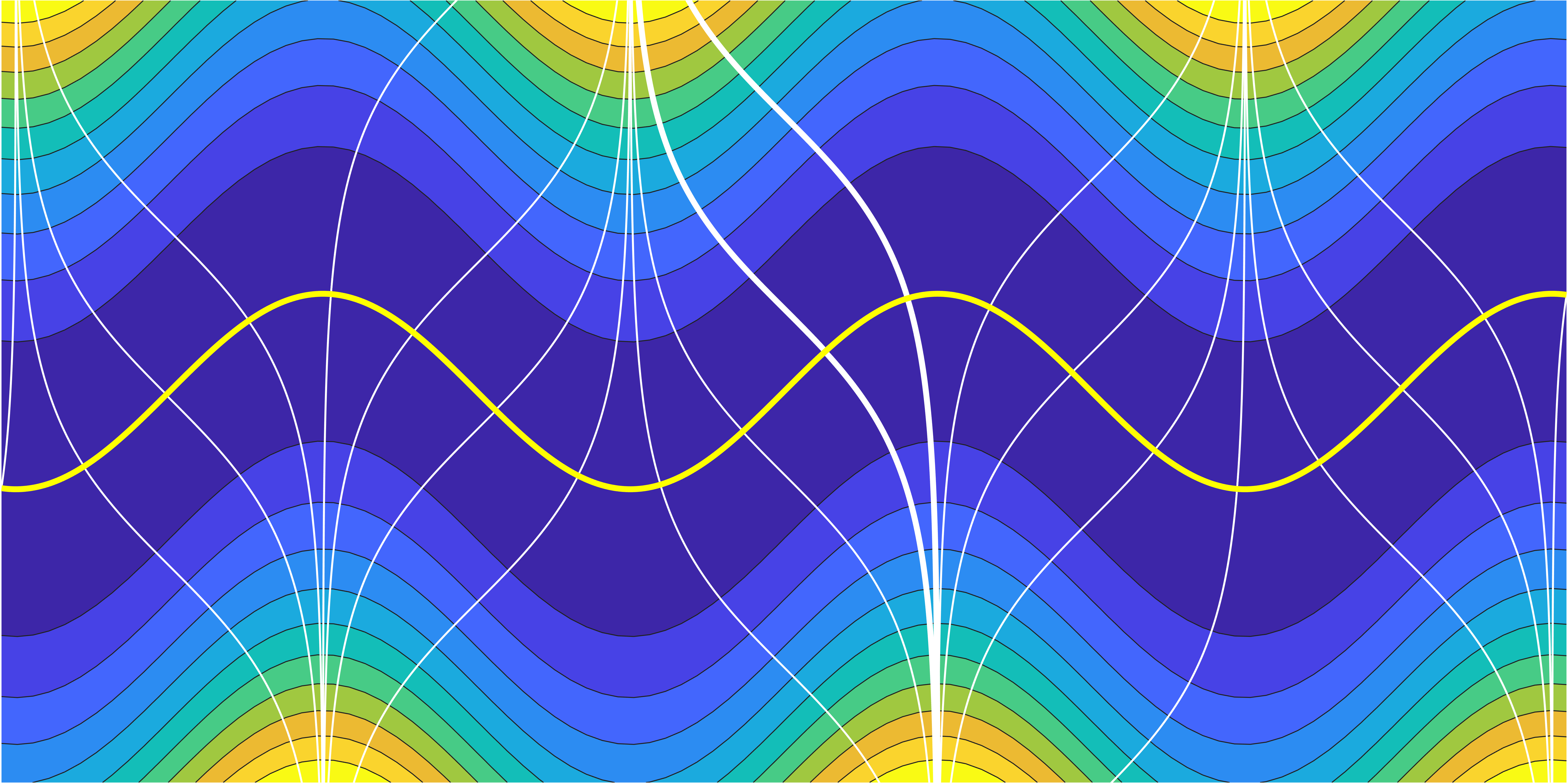
To prove Theorem 1, we must build a special diffeomorphism \(\psi = (\pi, \varphi) \colon \Rn \to S \times \Rk\). The idea is to “align” the “fibers” of the end-point map \(\pi\).

Fix a point \(x \in S\). Its fiber \(F\) is the set \[ F := \pi^{-1}(x) = \{y \in \Rn : \pi(y) = x \}. \] Since \(\pi \colon \Rn \to S\) is a smooth submersion (Lemma 5), this fiber is an embedded submanifold of \(\Rn\). Give \(F\) the Riemannian submanifold metric inherited from \(\Rn\).

For \(y \in F\), the fiber contains the entire gradient flow trajectory from \(y\) to \(x\). In particular, \(\nabla f(y)\) is tangent to \(F\) at \(y\). It is then easy to check that:

\(f|_F \colon F \to \reals\) is itself PŁ, and its unique minimizer is \(x\).

The Hessian of \(f|_F\) at \(x\) is positive definite (owing to PŁ). This provides a first piece of the puzzle:

Lemma 6 There exists a diffeomorphism \(\varphi_1 \colon F \to \Rk\) such that \(f(y) = f^* + \|\varphi_1(y)\|^2\).

Proof (sketch). Use the Morse Lemma to “rectify” \(f|_F\) near \(x\), then Palais–Cerf to extend this to a global diffeomorphism of \(F\). Follow up with normalized gradient flows (standard techniques in differential topology).

From here, the idea is to build a “nice” map \(\varphi_0 \colon \Rn \to F\) which should bring each point \(y \in \Rn\) (in any fiber) to some point in the reference fiber \(F\), in such a way that \[ f(\varphi_0(y)) = f(y). \] Indeed, if this is so, then we let \(\varphi = \varphi_1 \circ \varphi_0 \colon \Rn \to \Rk\) and observe \[ f(y) = f(\varphi_0(y)) = f^* + \|\varphi_1(\varphi_0(y))\|^2 = f^* + \|\varphi(y)\|^2, \] where the second equality holds because \(\varphi_0(y)\) is in \(F\).

Level sets of a PŁ function on \(\reals^2\). The set \(S\) is the orange sinusoid. White curves are fibers of \(\pi\). Also depicted: a guiding curve \(c\) from \(\pi(y)\) to \(x\) on \(S\), and its lift \(\gamma\) to an isocurve of \(f\) from \(y\) to \(\varphi_0(y)\).

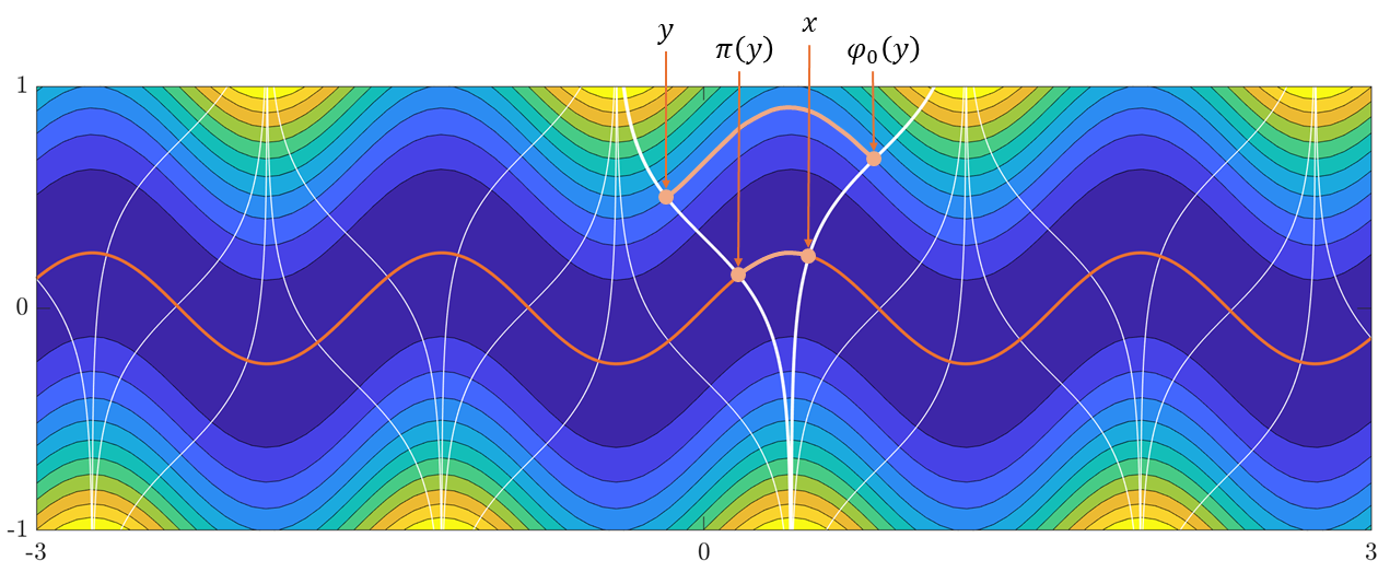
How can we build \(\varphi_0 \colon \Rn \to F\)? Here is the intuition:

1. Any given \(y \in \Rn\) belongs to some fiber, attached to \(\pi(y)\).

2. Choose a “guiding” curve \(c\) on \(S\) from \(c(0) = \pi(y)\) to \(c(1) = x\).

3. “Lift” \(c\) to a curve \(\gamma\) from \(\gamma(0) = y\) to “some point in \(F\)” \(\gamma(1)\) — we’ll call that \(\varphi_0(y)\).

4. Do this in a way that \(f\) remains constant along \(\gamma\), as then \[ f(y) = f(\gamma(0)) = f(\gamma(1)) = f(\varphi_0(y)), \] as desired.

Concretely, we choose the guiding curve as \[ c(t) = \pi\big((1-t) \pi(y) + tx\big). \] It depends (smoothly) on \(\pi(y)\).

The lifted curve should satisfy: \[\begin{align*} \gamma(0) & = y, \\ \pi(\gamma(t)) & = c(t) && \textrm{ for all } t \in [0, 1], \textrm{ and} \\ f(\gamma(t)) & = f(y) && \textrm{ for all } t \in [0, 1] \textrm{ (constant)}. \end{align*}\]

Notice this ensures \(\pi(\gamma(1)) = c(1) = x\), so \(\varphi_0(y) := \gamma(1)\) is indeed in \(F\).

To make these happen, we setup an ODE. In order to secure \(\pi \circ \gamma = c\), we need \[ \D\pi(\gamma(t))[\gamma'(t)] = c'(t). \] This is not enough to fix \(\gamma'(t)\) because \(\D\pi(\gamma(t))\) has a kernel. Specifically, that kernel is the tangent space to the fiber at \(\gamma(t)\). Now, we also want \(f \circ \gamma\) to be constant, hence \[ 0 = (f \circ \gamma)'(0) = \nabla f(\gamma(t))^\top \gamma'(0). \] Recall \(\nabla f(\gamma(t))\) is tangent to the fiber at \(\gamma(t)\). Thus, it makes sense to select \(\gamma'(t)\) orthogonal to the fiber.

Overall, we solve the following ODE, where \(\dagger\) denotes the Moore–Penrose pseudoinverse: \[\begin{align*} \gamma'(t) & = \D\pi(\gamma(t))^\dagger[c'(t)], \\ \gamma(0) & = y. \end{align*}\] This is a smooth ODE that depends smoothly on the parameter \(y\). It has a unique smooth solution, well defined for some interval of times.

To confirm that \(\gamma\) is defined for all \(t \in [0, 1]\), we rely on the Escape Lemma again: it notably says that the solution of the ODE exists for as long as it remains in a compact set.

To see that this is the case, we (finally!) use the fact that \(f\) is PŁ. Recall from Lemma 1 that gradient flow trajectories of \(f\) have bounded length. It follows that, for \(t \in [0, 1]\), \[\begin{align*} \|\gamma(t) - x\| & \leq \|\gamma(t) - c(t)\| + \|c(t) - c(1)\| \\ & \leq \|\gamma(t) - \pi(\gamma(t))\| + \ell(c) \\ & \leq \sqrt{\frac{2(f(\gamma(t)) - f^*)}{\mu}} + \ell(c) \\ & = \sqrt{\frac{2(f(y) - f^*)}{\mu}} + \ell(c), \end{align*}\] where \(\ell(c)\) is the length of the guiding curve \(c|_{[0, 1]}\).

This indeed confines \(\gamma|_{[0, 1]}\) to a ball around \(x\), with a radius that only depends on \(y\).

(Of course, many more details should be checked. In the paper, we notably verify that the resulting \(\psi = (\pi, \varphi)\) is indeed a diffeomorphism.)

What else is in the paper

In the paper, all proofs are worked out in detail, and there is far more discussion of literature and assumptions. In particular, some results do not require the full power of the \(C^\infty\) and global PŁ assumptions.

A more substantial distinction is this: in the paper, we start from a smooth PŁ function \(f \colon \calM \to \reals\) defined on a complete Riemannian manifold.

This brings the added question: in generalizing from \(\Rn\) to \(\calM\), which properties should we retain in order to preserve (variations of) the conclusions?

We found that pretty much all of the above works out as long as \(\calM\) is contractible (and we discuss what happens if it is not).

The general take requires a few extra layers of technicalities, which is why this blog post exists.

References

Ben Nejma, Aziz. 2025. “Polyak–Łojasiewicz Inequality Is Essentially No More General Than Strong Convexity for \(C^2\) Functions.” arXiv Preprint 2512.05285.

Calegari, Danny. 2019. “Wild Wild Whitehead.” Notices of the American Mathematical Society 66 (April): 1. https://doi.org/10.1090/noti1837.

Falconer, K. J. 1983. “Differentiation of the Limit Mapping in a Dynamical System.” Journal of the London Mathematical Society s2-27 (2): 356–72. https://doi.org/10.1112/jlms/s2-27.2.356.

Garrigos, Guillaume. 2023. “Square Distance Functions Are Polyak-Łojasiewicz and Vice-Versa.” https://arxiv.org/abs/2301.10332.

Glimm, James. 1960. “Two Cartesian Products Which Are Euclidean Spaces.” Bulletin de La Société Mathématique de France 88: 131–35. http://www.numdam.org/item?id=BSMF_1960__88__131_0.

Husch, L. S., and T. M. Price. 1970. “Finding a Boundary for a 3-Manifold.” Annals of Mathematics 91 (1): 223–35. http://www.jstor.org/stable/1970605.

Luft, E. 1987. “On Contractible Open 3-Manifolds.” Aequationes Mathematicae 34 (2-3): 231–39. https://doi.org/10.1007/BF01830674.

Mazur, Barry. 1961. “A Note on Some Contractible 4-Manifolds.” Annals of Mathematics 73 (1): 221–28. http://www.jstor.org/stable/1970288.

McMillan, D. R., and E. C. Zeeman. 1962. “On Contractible Open Manifolds.” Mathematical Proceedings of the Cambridge Philosophical Society 58 (2): 221–24. https://doi.org/10.1017/S0305004100036434.

Otto, F., and C. Villani. 2000. “Generalization of an Inequality by Talagrand and Links with the Logarithmic Sobolev Inequality.” Journal of Functional Analysis 173 (2): 361–400.

Perelman, Grigori. 2002--2003. “The Entropy Formula for the Ricci Flow and Its Geometric Applications; Ricci Flow with Surgery on Three-Manifolds; Finite Extinction Time for the Solutions to the Ricci Flow on Certain Three-Manifolds.” https://arxiv.org/abs/math/0211159, math/0303109, math/0307245.

Polyak, B. T. 1963. “Gradient Methods for the Minimisation of Functionals.” USSR Computational Mathematics and Mathematical Physics 3 (4): 864–78. https://doi.org/10.1016/0041-5553(63)90382-3.

Rebjock, Q., and N. Boumal. 2024. “Fast Convergence to Non-Isolated Minima: Four Equivalent Conditions for \(C^2\) Functions.” Mathematical Programming. https://doi.org/10.1007/s10107-024-02136-6.

Stallings, John. 1962. “The Piecewise-Linear Structure of Euclidean Space.” Proceedings of the Cambridge Philosophical Society 58 (3): 481–88. https://doi.org/10.1017/S0305004100036403.

Whitehead, J. H. C. 1935. “A certain open manifold whose group is unity.” The Quarterly Journal of Mathematics 1 (January): 268–79. https://doi.org/10.1093/qmath/os-6.1.268.