Designing polynomials for Muon’s polar factorization: focus on quintics

Let \(X \in \Rmn\) be a full rank, wide matrix, that is, with more columns than rows (\(m \leq n\)). If not, transpose.

The polar factor of \(X\) is the orthonormal matrix \(Q \in \Rmn\) (\(QQ\transpose = I_m\)) that is closest to \(X\) in the Frobenius norm. This is a standard concept in matrix analysis. In optimization, it is relevant for the metric projection retraction on the Stiefel manifold (which includes optimization over rotations). More recently, it became relevant in training LLMs with the Muon algorithm.

This post adds to a collection of proposals for how to approximate \(Q\) using only a few matrix-matrix multiplications.

Concretely, the user only needs to set one parameter: \(v_0 > 0\). From there, a sequence of degree-5 polynomials \(q_1, q_2, \ldots\) is generated. Applying them to (a scaled version of) \(X\) one after the other generates an approximation of \(Q\).

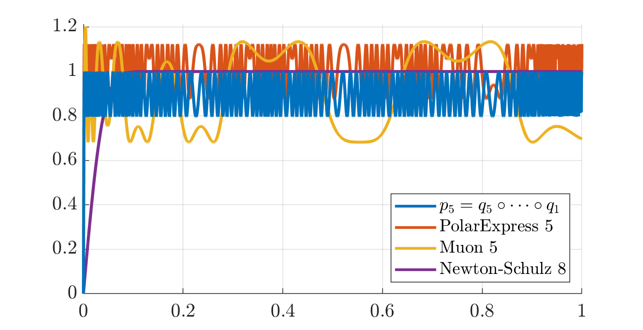
The next plot (and its zoomed version thereafter) builds the polynomial \(p_5 = q_5 \circ \cdots \circ q_1\) with \(v_0 = 10^{-3}\) and compares it with Muon’s quintic applied 5 times. A polynomial is deemed “better” if it maps more of \([0, 1]\) closer to \(1\).

We also compare with applying the first five quintics of the Polar Express paper: those are the minimax polynomials further tweaked for numerical stability. As it turns out (from discussions with the authors), the polynomials constructed in this post are the minimax polynomials too (before tweaking), but computed differently.

For higher accuracy, see tables of coefficients at the end.

The proposed polynomial \(p_5\) is a composition of \(5\) quintics, designed with \(v_0 = 10^{-3}\). This has the same computational cost as Muon’s proposal of applying a fixed quintic 5 times. These are further compared with applying the 5 first quintics of the Polar Express paper (optimal polynomial tweaked for stability). All of these require 15 matrix-matrix multiplications. Also shown is the result of applying Newton–Schulz’s cubic 8 times, for a total of 16 matrix-matrix multiplications.

Zoom of the previous plot to the interval \([0, 10^{-2}]\) on the horizontal axis. Polar Express has a faster initial rise while our polynomial stays below \(1\): this is part of a trade-off which can be changed—see the comparison section.

The task: approximate the polar factor on GPU

The polar factor can be computed explicitly from an SVD of \(X\), as follows. Let \(\sigma_1, \ldots, \sigma_m > 0\) denote the singular values of \(X\). Then, \[\begin{align*} X & = U \Sigma V\transpose, && U \in \Rmm, U\transpose U = I_m, \\ & && V \in \Rnm, V\transpose V = I_m, \\ & && \Sigma \in \Rmm, \Sigma = \diag(\sigma_1, \ldots, \sigma_m), \\ Q & = UV\transpose. \end{align*}\] On CPU, the SVD is hard to beat. On GPU, we may hope to get an advantage from algorithms that rely mostly on matrix-matrix multiplications. This is the topic of what follows, although it’s good to remember and compare with the SVD for matrices of the size you care about.

The old idea revisited recently is to approximate \(Q\) as a polynomial function of \(X\). Since \(X\) and \(Q\) should have the same (rectangular) size, dimensional considerations lead us to entertain only odd polynomials. Indeed, the “square” of \(X\), either \(XX\transpose\) or \(X\transpose X\), does not have the same size as \(X\). But the “cube” of \(X\), namely, \(XX\transpose X\), does. Likewise, any odd power \((XX\transpose)^d X\) (of degree \(2d+1\)) has the same size as \(X\), so we can add them up.

Specifically, if \(p(t) = c t^5 + b t^3 + a t\), then we let \[ p(X) = c (XX\transpose)^2 X + b (XX\transpose) X + a X. \] Computing \(p(X)\) is trivial (best done using Horner’s method), and very GPU friendly: it only requires 3 matrix-matrix multiplications.

Matlab

XXt = X*X';             % one mat-mat: (m x n) (n x m)
M = b*XXt + c*XXt*XXt;  % one mat-mat: (m x m) (m x m)
pX = a*X + M*X;         % one mat-mat: (m x m) (m x n)

PyTorch

XXt = X @ X.T                  # one mat-mat: (m x n) (n x m)
M = b * XXt + c * (XXt @ XXt)  # one mat-mat: (m x m) (m x m)
pX = a * X + M @ X             # one mat-mat: (m x m) (m x n)

Substituting the SVD \(X = U \Sigma V\transpose\) into the cubic term, notice that \[ (XX\transpose) X = (U\Sigma V\transpose V \Sigma\transpose U\transpose) U\Sigma V\transpose = U \Sigma \Sigma\transpose \Sigma V\transpose = U \Sigma^3 V\transpose. \] Thus, the SVD of the “cube” of \(X\) is the same as that of \(X\), only with the singular values \(\sigma_i\) replaced by their cubes \(\sigma_i^3\). Adding up the monomials of degree 1, 3 and 5, for the polynomial \(p\) above we find that \[ p(X) = U \begin{bmatrix} p(\sigma_1) & & \\ & \ddots & \\ & & p(\sigma_m) \end{bmatrix} V\transpose. \] In other words:

Applying the odd polynomial \(p\) to \(X\) effectively applies the polynomial \(p\) to its singular values, without the need to compute the SVD of \(X\) at all.

Since the polar factor \(Q = UV\transpose = UI_mV\transpose\) is the same as \(X\) only with its singular values replaced by 1, the task at hand is clear:

We should design an odd polynomial \(p\) such that \(p(t) \approx 1\) for all \(t > 0\).

Since \(p\) must be odd, we shall also have \(p(t) \approx -1\) for all \(t < 0\), and also \(p(0) = 0\). In other words, \(p\) should approximate the sign function. As a result, our task is closely related to that of computing the matrix sign function for square matrices.

Skipping over a ton of literature

This post offers one more take, motivated by recent activity surrounding the Muon optimizer and by the enduring importance of the Stiefel manifold in applications of Riemannian optimization. It builds on discussions with Timon Miehling in the summer of 2023.

It would be good to add more context and pointers to literature, because this is a classical topic in numerical analysis. See for example Higham’s book about functions of matrices: Chapter 5 is entirely devoted to computing the matrix sign function.

Nevertheless, here are just a few recent pointers:

• The Muon blog post proposed one quintic to apply 5 times.
• The squeezing 1-2% blog post runs a numerical search to find five quintics whose composition improves over Muon’s.
• The Polar Express paper from May 2025 proposes a minimax construction using Remez’s algorithm to find optimal quintics. They then tweak these polynomials in a principled way in order to improve numerical stability. Such considerations appear also in a paper by Chen and Chow, 2014 and by Nakatsukasa and Higham, 2012, who point out that applying the minimax polynomials is not backward stable. The Polar Express paper provides their final, tweaked coefficients explicitly, so we compare to those here.
• The Chebyshev paper from June 2025 also uses Remez’s algorithm to produce minimax polynomials. For cubics, they provide explicit expressions (see also Chen and Chow and the Polar Express paper for these). The authors further advocate using Gelfand’s formula to bound the operator norm. We did not run their code to compare with their polynomials, but they should be the (unique) minimax polynomials, so they should be the same as the (untweaked) Polar Express polynomials.

So what happens here? We provide a simple construction for quintics that is not (explicitly) based on the Remez algorithm. The construction is driven by heuristic arguments that made sense to us, and is easy to code. In particular, we wanted to build quintics that keep the singular values below 1 at all times (rather than oscillate around 1). In the end, they are minimax optimal (as argued by Noah Amsel). This is clear from the equioscillations in a narrow band below 1. After scaling to get symmetric oscillations around 1, our polynomials are equivalent to the minimax ones built using Remez.

Don’t hesitate to write with suggestions for other literature notes. We are grateful to the authors of Polar Express—David Persson, Robert Gower and Noah Amsel in particular—for many useful pointers that have been incorporated here.

Designing \(p\) as a product of polynomials

If \(p\) has degree \(2d+1\), then applying \(p\) to \(X\) requires \(d+1\) matrix-matrix multiplications, so we would rather keep the degree low. Another reason to stick to low degree polynomials is the risk of numerical issues: combining large powers of \(X\) is unlikely to work well in finite precision arithmetic, especially in the low precisions used for LLM training.

Yet, if \(p\) has low degree, then it won’t be a good approximation of the sign function. A classical alternative is to design a low-degree polynomial \(q\), then to apply it several times in succession. Say \(q\) has degree 5 for example. If we apply it \(k\) times, then \[ p = q \circ \cdots \circ q = q^k \] has degree \(5^k\). Applying \(q\) requires 3 matrix-matrix multiplications, for a total of \(3k\) mat-mats to apply \(p\)—pretty cheap for such a high degree polynomial.

The Newton–Schulz method does this with the cubic \(q(t) = -\frac{1}{2} t^3 + \frac{3}{2} t\).

The obvious next observation is that we are not forced to iterate the same \(q\) over and over. We may as well design a few low-degree polynomials \(q_1, \ldots, q_k\) and compose them: \[ p = q_k \circ \cdots \circ q_1. \] (Since polynomials commute, the ordering does not matter; but it will be convenient to think of them “in order”.)

As long as applying each polynomial to the output of the previous one is numerically stable (in some appropriate sense), then the overall procedure should behave well. More explicitly, upon applying \(q_1\) to \(X\), the singular values \(\sigma_i\) of \(X\) are mapped to \(q_1(\sigma_i)\)—so, \(q_1\) should behave well on the singular values. These numbers then pass through \(q_2\), so \(q_2\) should behave well on the new values \(q_1(\sigma_i)\).

To facilitate this, we first normalize \(X\) to have singular values in \([0, 1]\), then we design good polynomials for that interval.

Normalizing \(X\)

The polar factor of \(X\) is the same as the polar factor of \(\frac{1}{s}X\) for any scaling factor \(s > 0\). Thus, as is standard, we may apply our polynomial to \(\frac{1}{s}X\) rather than \(X\). If \(s\) is an upper bound on the largest singular value of \(X\), then the singular values of \(\frac{1}{s} X\) are all in \([0, 1]\), which is rather convenient: we assume so going forward.

How to compute such an upper bound on \(\sigma_1(X)\) (the operator norm of \(X\))? The Muon algorithm uses \(s = \frobnorm{X} + \epsilon\). We can improve on this as follows (perhaps also adding some \(\epsilon\)): \[ \sigma_1(X) \leq s := \min(\frobnorm{X}, \|XX\transpose\|_1^{1/2}) = \sqrt{\min(\trace(XX\transpose), \|XX\transpose\|_1)}, \] where the 1-norm of a matrix is the largest 1-norm of any of its columns. The inequality follows from \(\sigma_{1}(X) = \sqrt{\lambda_{\mathrm{\max}}(XX\transpose)}\) and Gershgorin’ circle theorem applied to \(XX\transpose\). It is cheap to compute \(s\) because \(XX\transpose\) must be computed anyway.

Notice that if \(X\) is already orthonormal, then \(s = \|XX\transpose\|_1^{1/2} = 1\), whereas the Frobenius norm is \(\sqrt{m}\). Thus, we would not scale an orthonormal matrix at all, which is sensible.

It may happen that \(\|XX\transpose\|_1 > \trace(XX\transpose)\): simply consider \(X = \begin{bmatrix} 1 & 0 \\ 2 & 2 \end{bmatrix}\) so that \(XX\transpose = \begin{bmatrix} 1 & 2 \\ 2 & 8 \end{bmatrix}\) has 1-norm \(10\) and trace \(9\).

See also this paper for another possible scaling based on Gelfand’s formula.

Designing the individual polynomials \(q_1, \ldots, q_k\).

Now that we can assume the singular values of \(X\) are in \([0, 1]\), we choose to stay in this interval.

Design each polynomial \(q_1, \ldots, q_k\) in such a way that it maps the interval \([0, 1]\) to \([0, 1]\).

The singular values of (the normalized) \(X\) are all less than 1, and hence the same is true of the singular values of \(q_1(X)\) then \(q_2(q_1(X))\) etc.

It makes sense to require this as well:

Design each polynomial \(q_1, \ldots, q_k\) such that \(q_j(1) = 1\).

This way, applying the polynomial to a matrix which is already orthonormal has no effect. (Recall that our proposed scaling also had this property.)

Finally, let us make the following judgment call:

Require each polynomial \(q_1, \ldots, q_k\) to have degree at most 5.

The rationale is that we want low, odd degrees; after some tinkering, degree 3 appears to be too low (but see also this paper), while degree 5 works well for Muon already with \(k = 5\).

\[ \newcommand{\trise}{t_{\mathrm{rise}}} \newcommand{\tmax}{t_{\mathrm{max}}} \newcommand{\tmin}{t_{\mathrm{min}}} \]

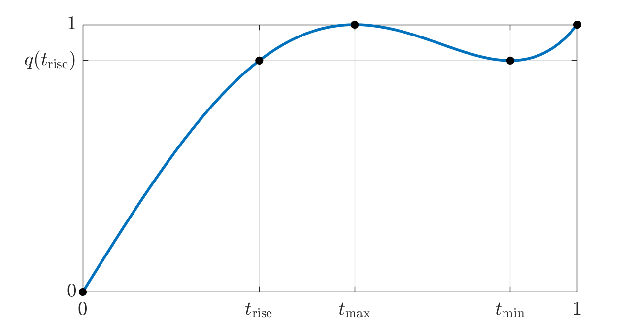
What do such polynomials look like? Let \[ q(t) = c t^5 + b t^3 + a t. \] To ensure \(q(1) = 1\), we need \[ a + b + c = 1. \] Let us also require \(q\) to attain the value \(1\) at some point \(\tmax \in [0, 1]\) which should be a local maximum. This way, \(q\) rises from \(q(0) = 0\) (since it’s odd) up to value 1 at \(\tmax\), then it decreases down to some value (we’ll want that to be positive), then it rises back up to \(q(1) = 1\). Effectively, we require \(q(\tmax) = 1\) and \(q'(\tmax) = 0\), that is, \[\begin{align*} c \tmax^5 + b \tmax^3 + a \tmax = 1, && 5 c \tmax^4 + 3 b \tmax^2 + a = 0. \end{align*}\] This is a total of 3 linear equations for the three coefficients \(a, b, c\): \[\begin{align*} \begin{bmatrix} 1 & 1 & 1 \\ \tmax & \tmax^3 & \tmax^5 \\ 1 & 3\tmax^2 & 5\tmax^4 \end{bmatrix} \begin{bmatrix} a \\ b \\ c \end{bmatrix} = \begin{bmatrix} 1 \\ 1 \\ 0 \end{bmatrix}. \end{align*}\] A quick investigation reveals the following:

For all \(\tmax \in [.36703, 1)\), the linear system above has a unique solution and the resulting polynomial \(q(t) = c t^5 + b t^3 + a t\) maps \([0, 1]\) to \([0, 1]\).

More precisely, the lower bound on \(\tmax\) is \(.367029487501048\). This results in a quintic that rises from \(0\) at \(t = 0\) to \(1\) at \(t = \tmax\), then decreases down to \(0\) at \(t \approx 0.8207\) and rises back up to \(1\) at \(t = 1\).

For \(\tmax < .36703\), the local minimum of \(q\) in the interval \([0, 1]\) drops below \(0\), so that \(q\) does not map \([0, 1]\) to \([0, 1]\). For \(\tmax \to 1\), the polynomial tends to \(q(t) = \frac{3}{8} t^5 - \frac{5}{4} t^3 + \frac{15}{8} t\).

Example polynomial \(q(t) = c t^5 + b t^3 + a t\) designed to satisfy \(q(1) = 1\) and to have a local maximum at \(\tmax = .55\) with value 1. The local minimum is found at \(\tmin \approx .864\), with value \(v := q(\tmin) \approx .865\). The first \(t\) at which \(q\) attains the value \(v\) is \(\trise \approx .357\). Notice how \(q\) maps (“compresses”) the interval \([\trise, 1]\) to \([q(\trise), 1]\).

A closer look at these quintics

In designing each of the polynomials \(q\), we have a trade-off to make. On the one hand, it should rise quickly so that singular values near 0 quickly increase toward the target 1. This would have us take \(\tmax\) small. On the other hand, larger singular values should not be dragged down. This would have us take \(\tmax\) larger.

Here is one fruitful way to think about the trade-off. For each \(\tmax\) in the stated interval, we get an associated polynomial \(q\) and we can define the following interesting values of \(t\): \[ 0 < \trise < \tmax < \tmin < 1, \] where:

• \(\tmax\) is the (chosen) location of the local maximum, designed such that \(q(\tmax) = 1\);
• \(\tmin\) is the location of the local minimum, with value \(v := q(\tmin) \geq 0\);
• \(\trise\) is the earliest time where \(q\) attains the local minimum value, so that \(q(\trise) = q(\tmin) = v\).

Notice that \(q\) maps the interval \([\trise, 1]\) to the interval \([v, 1] = [q(\trise), 1]\). If the latter is narrower than the former (that is, if \(q(\trise) > \trise\), which is indeed the case), then we effectively “compress” the former range of values to be closer to 1, uniformly.

The coefficients \(a, b, c\) to form \(q\) and the numbers \(\trise, \tmin, v\) are all computed from \(\tmax\) in the Matlab code below (translated to Python with ChatGPT).

Matlab

function [q, trise, v, tmin] = qdesign(tmax)
    assert(tmax > 0 && tmax <= 1);
    if tmax < 1-1e-7 % solve a linear system for (a, b, c).
        abc = [   1,        1,        1
               tmax,   tmax^3,   tmax^5
                  1, 3*tmax^2, 5*tmax^4] \ [1 ; 1 ; 0];
        q = [abc(3), 0, abc(2), 0, abc(1), 0];
    else % unless tmax is numerically too close to 1.
        q = [3/8, 0, -5/4, 0, 15/8, 0]; % this is the limit for tmax -> 1.
    end
    tmin = max(roots(polyder(q))); % find the positive local min of q.
    v = polyval(q, tmin); % evaluate v = q(tmin).
    if v >= 0
        % find the earliest positive time trise s.t. q(trise) = q(tmin).
        q_equals_v = roots(q - [0, 0, 0, 0, 0, v]);
        trise = min(q_equals_v(abs(imag(q_equals_v)) < 1e-8 & real(q_equals_v) > 0));
    else
        % triggers for tmax < .367029487501048
        trise = nan;
    end
end

Python

import numpy as np
from numpy.polynomial import Polynomial

# Call this as: q, trise, v, tmin = qdesign(tmax)
def qdesign(tmax):
    assert 0 < tmax <= 1, "tmax must be in (0, 1]"

    if tmax < 1 - 1e-7:
        A = np.array([
            [1, 1, 1],
            [tmax, tmax**3, tmax**5],
            [1, 3*tmax**2, 5*tmax**4]
        ])
        rhs = np.array([1, 1, 0])
        abc = np.linalg.solve(A, rhs)
        q_coeffs = np.array([0, abc[0], 0, abc[1], 0, abc[2]])
    else:
        q_coeffs = np.array([0, 15/8, 0, -5/4, 0, 3/8])

    q = Polynomial(q_coeffs)

    dq = q.deriv()
    tmin_candidates = dq.roots().real.max()
    v = q(tmin)

    if v >= 0:
        q_minus_v = q - v
        trise_candidates = q_minus_v.roots()
        trise_candidates = trise_candidates[np.isreal(trise_candidates)].real
        trise_candidates = trise_candidates[trise_candidates > 0]
        trise = trise_candidates.min()
    else:
        trise = np.nan

    return q, trise, v, tmin

Bootstrapping a good trade-off

The properties above suggest the following strategy:

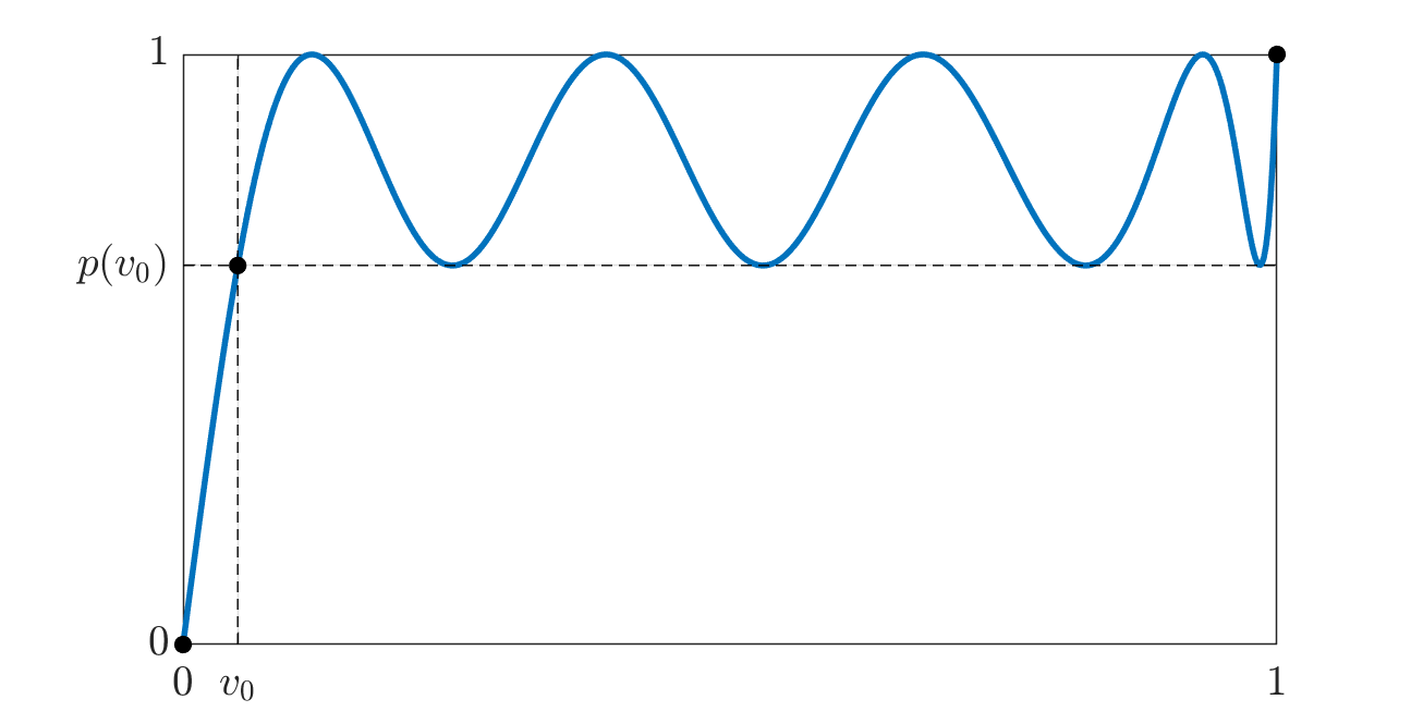
1. Assume all the singular values of \(X\) (potentially after scaling) are in the interval \([v_0, 1]\) for some \(v_0 > 0\).
2. Find \(\tmax\) such that \(\trise = v_0\) (this requires solving one not-too-bad nonlinear equation, see below).
3. From this \(\tmax\), we get a first polynomial: \(q_1\).
4. Notice that \(q_1\) maps the interval \([v_0, 1]\) to \([v_1, 1]\) with \(v_1 = q_1(\trise) = q_1(v_0)\).
5. Repeat to produce \(q_2\) which further maps the interval to \([v_2, 1]\) with \(v_2 = q_2(v_1) = q_2(q_1(v_0))\), etc.
6. Overall, the composed polynomial \(p = q_k \circ \cdots \circ q_1\) maps the interval \([v_0, 1]\) to the interval \([p(v_0), 1]\), so that all singular values of \(p(X)\) are in the latter interval.

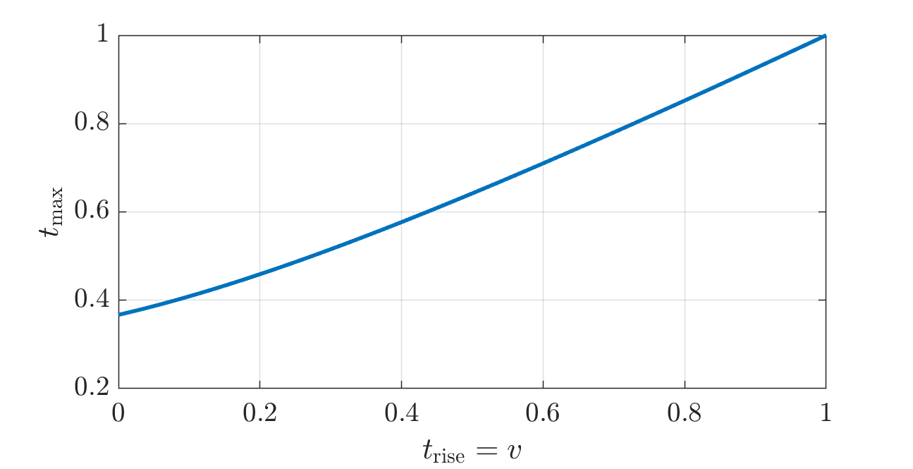
The code above already provides the function \(\tmax \mapsto \trise\): see figure below. The proposed procedure requires the inverse map, \(\trise \mapsto \tmax\): see the figure thereafter. The Matlab code below computes that inverse using just a few iterations of the secant method (again translated to Python with ChatGPT).

Matlab

% The function tmax -> trise is implemented in qdesign.
function trise = trisefun(tmax)
    [~, trise, ~, ~] = qdesign(tmax);
end
% This function provides the inverse relation, trise -> tmax.
function tmax = tmaxfun(trise)
    if trise <= .001 % good linear fit for small trise
        tmax = 0.37095592*trise + .367029487501048;
    elseif trise < .999
        % Use a secant method to solve trisefun(tmax) = trise.
        h = @(t) trisefun(t) - trise;  % want a root of h
        tt = [0.36703, .999];
        hh = [h(tt(1)), h(tt(2))];
        while abs(hh(end)) > 1e-8   % takes <= 6 iterations
            num = tt(end-1)*hh(end) - tt(end)*hh(end-1);
            den = hh(end) - hh(end-1);
            tt(end+1) = num / den;
            hh(end+1) = h(tt(end));
        end
        tmax = tt(end);
    else % good linear fit for large trise
        tmax = .75*trise + .25;
    end
end

Python

def tmaxfun(trise):
    if trise <= 0.001:
        # Good linear fit for small trise
        return 0.37095592 * trise + 0.367029487501048
    elif trise < 0.999:
        # Use secant method to find tmax such that trise(tmax) = trise,
        # that is, find a root of h(t).
        def h(t):
            _, trise_of_t, _, _ = qdesign(t)
            return trise_of_t - trise

        tt = [0.36703, 0.999]
        hh = [h(tt[0]), h(tt[1])]

        while abs(hh[-1]) > 1e-8:
            num = tt[-2] * hh[-1] - tt[-1] * hh[-2]
            den = hh[-1] - hh[-2]
            tt.append(num / den)
            hh.append(h(tt[-1]))

        return tt[-1]
    else:
        # Good linear fit for large trise
        return 0.75 * trise + 0.25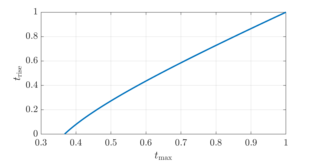

From a given \(\tmax\) in the range \([.367, 1]\), we can easily compute \(\trise\). The resulting function \(\tmax \mapsto \trise\) is plotted here. To design our polynomials, we need to invert that function, that is, given a \(\trise\), we must find the associated \(\tmax\). See the next plot.

Given a \(v\) in the range \((0, 1)\), we solve the (gentle) nonlinear equation \(\trise(\tmax) = v\) using about 6 iterations of the secant method. This provide access to the inverse map \(\trise \mapsto \tmax\).

An example

Let’s do an example.

1. Set \(v_0 = 10^{-3}\) (this is the only parameter).
2. Use the secant method to find \(\tmax = .367400\), which is such that \(\tmin(\tmax) = v_0\).
3. The corresponding polynomial is \(q_1(t) = 9.35426 t^5 - 12.6074 t^3 + 4.25318 t\).
4. Compute \(v_1 = q_1(v_0) = 0.004253\).
5. Use the secant method to find the next \(\tmax = 0.368614\), such that \(\tmin(\tmax) = v_1\).
6. The corresponding polynomial is \(q_2(t) = 9.25866 t^5 - 12.4989 t^3 + 4.24023 t\).
7. Compute \(v_2 = q_2(v_1) = 0.018033\).
8. …

Here is the Matlab code and its Python translation.

Matlab

% Decide how narrow the burn-in band should be.
v0 = 1e-3;
% Choose how many polynomials $q_1, q_2, ...$ to design.
npols = 8;

vv = zeros(1, npols+1); % values $v_0, v_1, ..., v_{npols}$
qq = zeros(6, npols);   % qq(:, k) holds the coefficients of $q_k$
vv(1) = v0;             % and $v_1$ = vv(2), $v_2$ = vv(3), ...
for counter = 1 : npols
    v = vv(counter);
    tmax = tmaxfun(v);  % solve the nonlinear equation
    q = qdesign(tmax);  % design the polynomial for this $t_\max$
    qq(:, counter) = q';
    vv(counter+1) = polyval(q, v);
end

Python

v0 = 1e-3
npols = 8

qq = np.zeros((6, npols))  # columns hold coefficients for q_1, q_2, ...
vv = np.zeros(npols + 1)   # holds values v0, v1, ..., v_npols
vv[0] = v0

for counter in range(npols):
    v = vv[counter]
    tmax = tmaxfun(v)            # solve nonlinear equation for this v
    q, _, _, _ = qdesign(tmax)   # get polynomial q (Polynomial object)
    qq[:, counter] = q.coef[:6]  # extract its coefficients
    vv[counter + 1] = q(v)       # and evaluate it at v


print("  k   v_k                   Coefficients of q_k (degrees 1, 3, 5)")
print("---------------------------------------------------------")
print(f"{0:3d}  {vv[0]: .16f}")
for k in range(npols):
    coeffs = "  ".join(f"{c: .16f}" for c in qq[[1, 3, 5], k])
    print(f"{k+1:3d}  {vv[k+1]: .16f}   {coeffs}")

Below are the coefficients this produces for the choice \(v_0 = 10^{-3}\), together with the associated values \(v_1, \ldots, v_8\). These mean that if we apply the polynomial \(p_k := q_k \circ \cdots \circ q_1\) to a matrix \(X\) whose singular values are all in the interval \([v_0, 1]\), then the resulting matrix \(p_k(X)\) has all of its singular values in the interval \([v_k, 1]\) (which quickly compresses to being almost just 1).

Because the polynomials individually map \([0, 1]\) to \([0, 1]\), we also know that if \(X\) has some singular values below \(v_0\), then these remain in \([0, 1]\) as well. In fact, they too get much closer to 1, because \(p_k'(0) = q_k'(0) \cdots q_1'(0)\) is the product of the first \(k\) coefficients of the monomial \(t\): this grows fast.

                     t^5                   t^3                    t                v
                                                                       0.001 (input)
q_1:   9.354261375134167,  -12.607439558244193,   4.253178183110027,   0.00425
q_2:   9.258657278862632,  -12.498887938250022,   4.240230659387390,   0.01803
q_3:   8.858706841516742,  -12.043821651987571,   4.185114810470829,   0.07540
q_4:   7.301830255047141,  -10.255723292283191,   3.953893037236051,   0.29375
q_5:   3.300045676834200,   -5.456882096891140,   3.156836420056940,   0.79622
q_6:   0.643782951067994,   -1.744845423174929,   2.101062472106936,   0.99817
q_7:   0.376721636882429,   -1.253440908236615,   1.876719271354186,   0.9999999990
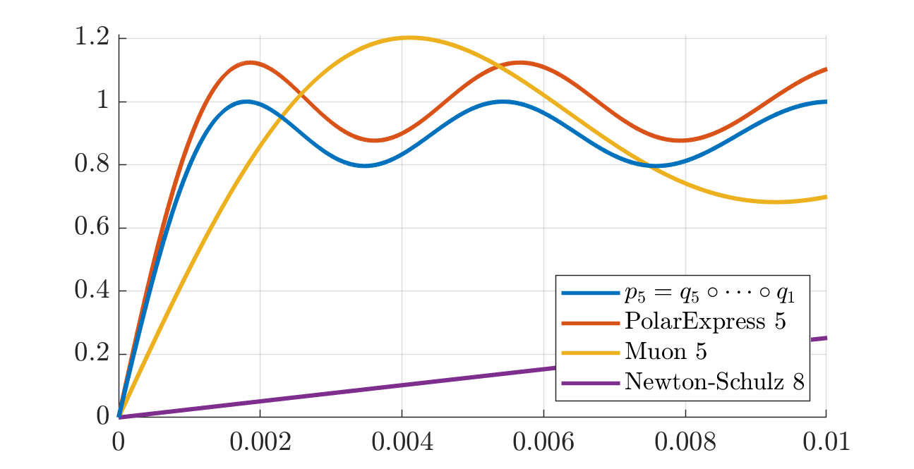
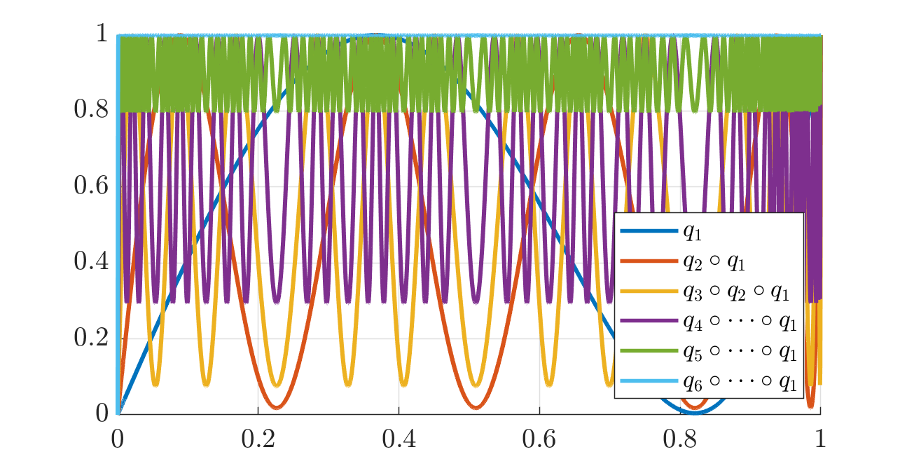
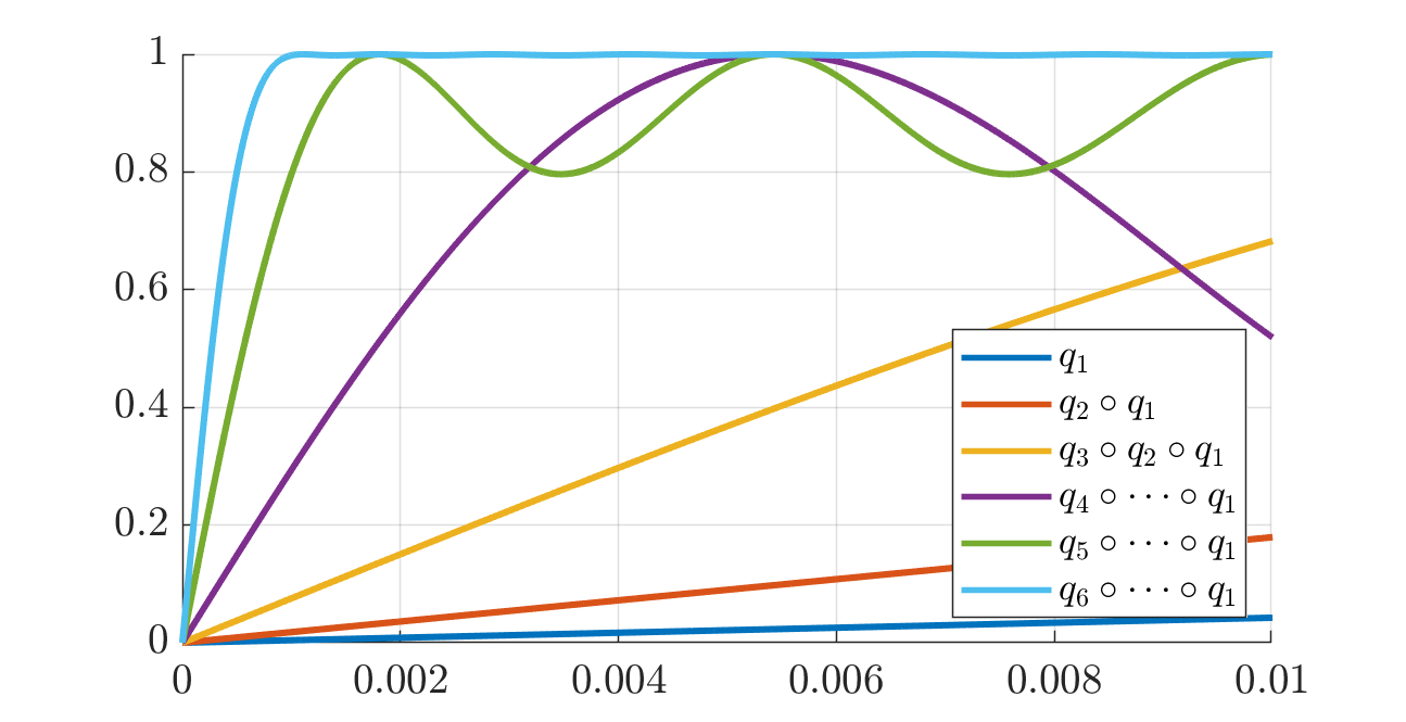
q_8:   0.375000000000000,   -1.250000000000000,   1.875000000000000,   numerically 1

The corresponding progression of polynomials \(q_1, q_2 \circ q_1, q_3 \circ q_2 \circ q_1\) etc. is displayed in the next two figures: the second one is a zoom of the first so as to better see the initial rise of the polynomials on the interval \([0, 10^{-2}]\).

For \(v_0 = 10^{-3}\), these are the proposed polynomials \(p_1 = q_1\), \(p_2 = q_2 \circ q_1\), \(p_3 = q_3 \circ q_2 \circ q_1\) up to \(p_6 = q_6 \circ \cdots \circ q_1\). Applying \(p_k\) to a matrix requires \(3k\) matrix-matrix multiplications.

Zoom of the previous plot to better see the interval \([0, 10^{-2}]\) on the horizontal axis. Look at \(q_5 \circ \cdots \circ q_1\) in particular: notice how it reaches its “ripple” level exactly at \(t = 10^{-3} = v_0\), as intended.

Comparison to Muon and others

The two plots at the very top of this post illustrate the polynomial \(p_5 = q_5 \circ \cdots \circ q_1\) with \(v_0 = 10^{-2}\) as compared to Muon and Polar Express.

We forced our polynomials to map 1 to 1 (so that applying them to an orthonormal matrix has no effect) and to map \([0, 1]\) to \([0, 1]\) (which is intuitively desirable for numerical reasons). If one does not particularly care about either, then one might instead prefer polynomials that are as close as possible to \(1\), regardless of over- or under-shooting.

Since our polynomial \(p_k = q_k \circ \cdots \circ q_1\) maps \([v_0, 1]\) to \([v_k, 1]\), one way to exploit the new leeway is to multiply \(p_k\) by \(\alpha_k\) so that it oscillates in \([\alpha_k v_k, \alpha_k]\). This is centered around \(1\) if we let \(\alpha_k = \frac{2}{1+v_k}\). The next plot (and its zoomed version thereafter) is the same as above, but with our \(p_5\) rescaled in this fashion.

The equioscillations show that the rescaled \(p_5\) is the minimax optimal approximation of the sign function over some interval. The Polar Express paper builds its polynomials using Remez’s algorithm to produce minimax polynomials, and then tweaks them in several ways to improve numerical stability, which is especially important in the context of the Muon algorithm that is normally run in low-precision arithmetic. This is why their polynomial does not quite equioscillate and the amplitude of the oscillations is a tad larger. Of course, removing those safety factors in their construction restores optimality.

Same plot as at the top of this post, but our polynomial was multiplied by \(\frac{2}{1+v_5} = 1.11344841\) so that it oscillates symmetrically above and below 1.

Zoom of the previous plot.

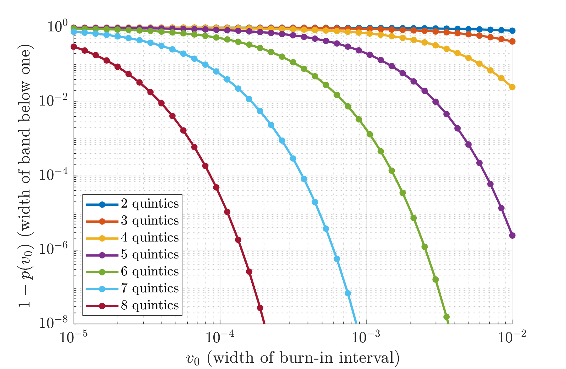
Trade-off curves

The code above makes it easy to explore how we can trade the following quantities:

• To use fewer matrix-matrix multiplications, apply fewer quintics.
• To effectively map small singular values close to 1, use a smaller \(v_0\).
• To make the mapped values really close to 1, arrange for \(p(v_0)\) to be really close to 1.

Of course, there is a give and take. The plot below shows exactly which trades can be made.

Upon choosing \(v_0\), we get quintics \(q_1, q_2, q_3, \ldots\) We decide to apply \(k\) of them, resulting in a polynomial \(p_k = q_k \circ \cdots \circ q_1\). It maps the interval \([v_0, 1]\) to \([p_k(v_0), 1]\). Naturally, we would like to make \(p_k(v_0)\) really close to \(1\), while also having \(v_0\) really close to \(0\), that is, we want to go “bottom left” in the plot. But we also want \(k\) small because applying \(p_k\) requires \(3k\) mat-mats. This plot shows which trade-offs can actually be achieved with the proposed method.

Illustration with just \(2\) quintics using the rather large \(v_0 = 0.05\), to make the roles of \(v_0\) and \(p(v_0)\) clearly visible in the resulting polynomial \(p_2 = q_2 \circ q_1\). Ideally, we want \(v_0 \approx 0\) and \(p(v_0) \approx 1\).

More tables of coefficients

Above, the coefficients are given for the polynomials designed with \(v_0 = 10^{-3}\). Here are the numbers for various values of \(v_0\) from \(10^{-1}\) to \(10^{-6}\). The first three numbers in each row specify one odd polynomial of degree 5. See above for interpretation of the last column.

\(v_0 = 10^{-1}\)

                 t^5                 t^3                   t                   v
                                                               0.100000000000000
   6.696917332243658  -9.552448753532390   3.855531421288732   0.376067662548663
   2.453346766199894  -4.367376132943869   2.914029366743975   0.882042532579576
   0.508746117946840  -1.505371230293261   1.996625112346422   0.999691899945929
   0.375288985412072  -1.250577904041234   1.875288918629162   0.999999999995429
   0.375000000000000  -1.250000000000000   1.875000000000000   1.000000000000000

\(v_0 = 10^{-2}\)

                 t^5                 t^3                   t                   v
                                                               0.010000000000000
   9.090846367051181 -12.308141435465149   4.217295068413968   0.042160643451789
   8.180852172219334 -11.268785908085340   4.087933735866006   0.171506508085117
   5.170659597990138  -7.749714190101462   3.579054592111324   0.575502861111208
   1.249716292114231  -2.702225182665636   2.452508890551405   0.975253448959634
   0.399105644591936  -1.297761493281863   1.898655848689927   0.999997541854788
   0.375008560632811  -1.250017121215238   1.875008560582427   1.000000000000000
   0.375000000000000  -1.250000000000000   1.875000000000000   1.000000000000000

\(v_0 = 10^{-3}\)

                 t^5                 t^3                   t                   v
                                                               0.001000000000000
   9.354254438089731 -12.607431684816314   4.253177246726583   0.004253164639304
   9.258657306317708 -12.498887969435600   4.240230663117892   0.018033437501851
   8.858706955036302 -12.043821781375303   4.185114826339001   0.075401391818523
   7.301830666972178 -10.255723769380129   3.953893102407951   0.293750366356853
   3.300046357967521  -5.456882956513900   3.156836598546380   0.796221449716703
   0.643783084212975  -1.744845652381765   2.101062568168790   0.998168733986030
   0.376721638904215  -1.253440912274638   1.876719273370423   0.999999999037802
   0.375000000000000  -1.250000000000000   1.875000000000000   1.000000000000000

\(v_0 = 10^{-4}\)

                 t^5                 t^3                   t                   v
                                                               0.000100000000000
   9.380771697141862 -12.637525071686762   4.256753374544900   0.000425675324817
   9.371164803090032 -12.626623339154714   4.255458536064681   0.001811442720666
   9.330370118052681 -12.580320738238134   4.249950620185453   0.007698467337738
   9.157884476562693 -12.384374335341327   4.226489858778635   0.032531843878649
   8.447677737242927 -11.574459819363790   4.126782082120863   0.133853639652915
   5.931204659112348  -8.653715217047411   3.722510557935063   0.477772856025335
   1.724237062972631  -3.382352208908426   2.658115145935795   0.944021257637481
   0.432297062770878  -1.362159809920564   1.929862747149686   0.999970146991013
   0.375028029395179  -1.250056058160037   1.875028028764858   0.999999999999996
   0.375000000000000  -1.250000000000000   1.875000000000000   1.000000000000000

\(v_0 = 10^{-5}\)

                 t^5                 t^3                   t                   v
                                                               0.000010000000000
   9.383428819087083 -12.640540176036508   4.257111356949425   0.000042571113557
   9.382467089836421 -12.639448884734739   4.256981794898318   0.000181224454425
   9.378374504132060 -12.634804859469307   4.256430355337248   0.000771369193743
   9.360981445612703 -12.615066514943244   4.254085069330541   0.003281464380077
   9.287167284307298 -12.531267961224923   4.244100676917625   0.013926422409997
   8.977017353933988 -12.178599670634693   4.201582316700705   0.058480120883865
   7.740814637072388 -10.762866834315677   4.022052197243289   0.233062845692248
   4.122882561490811  -6.480345671581840   3.357463110091029   0.703296568748728
   0.842267620475804  -2.074938794982717   2.232671174506913   0.993348242574019
   0.381300047426239  -1.262568619451921   1.881268572025682   0.999999953551545
   0.375000000000000  -1.250000000000000   1.875000000000000   1.000000000000000

\(v_0 = 10^{-6}\)

                 t^5                 t^3                   t                   v
                                                               0.000001000000000
   9.383694585333554 -12.640841744223408   4.257147158889854   0.000004257147159
   9.383598402001448 -12.640732603903782   4.257134201902334   0.000018123246772
   9.383188951437143 -12.640267994742334   4.257079043305191   0.000077152093953
   9.381446155994814 -12.638290403594974   4.256844247600160   0.000328424441529
   9.374032200542011 -12.629877300021391   4.255845099479380   0.001397723102622
   9.342544505180395 -12.594140473137385   4.251595967956989   0.005942519517496
   9.209182999551556 -12.442679696165410   4.233496696613853   0.025155025701497
   8.655477562994927 -11.811972489632256   4.156494926637329   0.104368807058658
   6.593720469562035  -9.431911058254771   3.838190588692736   0.389946138150438
   2.335790997472655  -4.212129843000478   2.876338845527824   0.892921341063178
   0.494201494400777  -1.478616710359919   1.984415215959143   0.999773520718532
   0.375212401438779  -1.250424766796637   1.875212365357858   0.999999999998185
   0.375000000000000  -1.250000000000000   1.875000000000000   1.000000000000000

Code for using those tables

Simply copy-paste one of the tables above (or compute a new one) into the code below. This won’t shine on CPU compared to the SVD, but you might like what it’s doing on GPU in low precision if that’s enough for your usage. Notice that further steps should be taken to make this stable in low precision: see the Polar Express paper for that.

function X = mypolarfactor(X)
% Input:  real matrix X of size m x n.
% Output: real matrix of size m x n that approximates polar factor of X.

    % Decide how many polynomials to apply (npols >= 1).
    npols = 5;

    % By default, all singular values of the output X are <= 1.
    % We can also choose to symmetrize the error by scaling X up.
    % If so, the singular values of X may be both above and below 1, but
    % potentially closer to 1 in absolute value.
    symmetrize = false;


    % Compute or copy-paste table of coefficients here.
    % Each row is a polynomial: q_1, q_2, ...
    % Columns 1, 2, 3 hold the coefficients for t^5, t^3, t^1.
    % Column 4 contains v_k (details in blog post).
    coeffs = [ ...
        9.354254438089731, -12.607431684816314,   4.253177246726583   0.004253164639304
        9.258657306317708, -12.498887969435600,   4.240230663117892   0.018033437501851
        8.858706955036302, -12.043821781375303,   4.185114826339001   0.075401391818523
        7.301830666972178, -10.255723769380129,   3.953893102407951   0.293750366356853
        3.300046357967521,  -5.456882956513900,   3.156836598546380   0.796221449716703
        0.643783084212975,  -1.744845652381765,   2.101062568168790   0.998168733986030
        0.376721638904215,  -1.253440912274638,   1.876719273370423   0.999999999037802
        0.375000000000000,  -1.250000000000000,   1.875000000000000   1.000000000000000
    ];

    transpose = false;
    if size(X, 1) > size(X, 2)
        X = X';
        transpose = true;
    end

    % Applying the first polynomial is a bit special,
    % because we still need to normalize X.
    % The normalization involves computing X*X', which
    % we want to recycle to apply the first polynomial.
    XXt = X*X';
    % Compute an upper bound s = sqrt(s2) on operator norm of X.
    s2 = min(trace(XXt), norm(XXt, 1));
    X = X/sqrt(s2);
    XXt = XXt/s2;
    M = coeffs(1, 2)*XXt + coeffs(1, 1)*XXt*XXt;
    X = coeffs(1, 3)*X + M*X;
    % X is now q_1(X/s).
    
    for k = 2 : npols
        % If we want to apply more polynomials than are provided,
        % we repeat the last one.
        kk = min(k, size(coeffs, 1));
        XXt = X*X';
        M = coeffs(kk, 2)*XXt + coeffs(kk, 1)*XXt*XXt;
        X = coeffs(kk, 3)*X + M*X;
    end

    if symmetrize && npols <= size(coeffs, 1)
        X = X * 2/(1+coeffs(npols, 4));
    end

    if transpose
        X = X';
    end

end